Let’s talk about the modern generative AI workhorse – the stable diffusion AI generator model. This blog post aims to provide information on how to train and use a stable diffusion AI image generator and what the process looks like from a developer’s perspective.
Stable Diffusion is an algorithm that generates high-quality images based on a text description. In this blog post, we focus on an intuitive explanation of the algorithm from the point of view of a deep learning developer. Note that the version of the algorithm described here is implemented in the popular library diffusers provided by Hugging Face.
Examples
Let’s start with examples of Stable Diffusion in action. Here are some input text/output image pairs from the Lexica website. These were generated using the “Lexica Aperture v2” version of the Stable Diffusion model.
“a photo of a beautiful black woman with black curly hair, dreamy, nostalgic, fashion editorial, studio photography, magazine photography, earth tones, 9:16”: | “Cute chibi cat dancing”: |
“pixel art san francisco fisherman’s Wharf. 3d pixel art 4k wallpaper. incredible pixel art details. flowers. pixel art. lots of people in foreground”: | “Darth Vader on trial, courtroom sketch, black and white” |
“pixel art san francisco fisherman’s wharf. 3d pixel art 4k wallpaper. incredible pixel art details. flowers. pixel art. lots of people in foreground”: | “simple vector line drawing, the outline of a woman sitting on a swing reading a book, clean vector daytime, tree, illustration, 6 colors, paper, vintage”: |
As we can see, the model is quite versatile in the images it can generate, which can vary significantly with respect to its subject and style.
About the model
Now for some basics on what a Stable Diffusion model really is (mostly from [Wikipedia]):
- Published in 2022.
- Developed by the startup Stability AI in collaboration with the CompVis group at the Ludwig Maximilian University of Munich, startup Runway, and others.
- Size: 4-8 GB (depending on the version)
- Trained on billions of image-caption pairs taken from LAION-5B, a publicly available dataset derived from Common Crawl, using 256 Nvidia A100 GPUs on AWS at a cost of $600k.
- Predecessors and direct competition: DALL-E from OpenAI, Imagen from Google. Note that both of these algorithms/services do the bulk of their processing in pixel space which is much more computationally demanding than the approach using lower-dimensional latent space as is done in Stable Diffusion. More on that later.
Main idea
Let’s consider a hypothetical process of adding noise to an image. A small amount of noise is added in consecutive time steps until we get an image of pure random noise, i.e., consisting entirely of pixels with assigned random values. This is called the diffusion process. We want to reverse this process, i.e., take an image consisting only of noise and predict what a slightly less noisy image might look like. We would then repeat this in consecutive time steps until a full image without noise is produced. This is shown in the following diagram (from [4, Fig. 2]):

To reverse the diffusion process, we need a model trained to remove noise from images. This model would receive a noisy image as input and produce a slightly less noisy image as an output. In practice, we usually use a model to predict just the noise in an image and then use this prediction to calculate how a slightly less noisy image would look in a separate step.
A natural question arises here: why don’t we predict an image without noise in a single step instead of doing it in many steps? The answer is that such an approach doesn’t work well in practice. This is because trying to predict anything from a very noisy image right away is very difficult (more on that later).
Let’s now consider what the desired properties of a model are for removing noise from images and how they can be achieved in practice.
- First, the model should do the bulk of its processing on scaled-down versions of the original images to make processing more computationally efficient. To do that, we want to “depart” from high-dimensional pixel space to lower-dimensional “latent space” and then return at the end of the process. These scaled-down images are called latent images.
- We’re going to use a popular model that allows us to go from pixel space to latent space and back: the Variational Autoencoder (VAE).
- The second property is that for a given (latent) input image, the model should predict the level of noise for each pixel for each channel (afterward, we’re going to subtract the predicted noise from the image to get a denoised image)
- Here we’re going to use a popular model that transforms an image into a different image of the same size: U-Net.
An important detail related to the diffusion process is the noise schedule. This is the level of noise (a.k.a. sigma, a.k.a. standard deviation of normal distribution) added to the image depending on the time step, a.k.a. t, during the diffusion process. Namely, we add random numbers coming from the normal distribution with a given sigma parameter to each pixel value in each channel of an image. An example noise schedule is presented in the image below.

In the diagram, t=0 corresponds to a fully denoised image, and t=T=1000 corresponds to an image consisting of pure noise.
Training
Now let’s focus on the details of the training phase of a Stable Diffusion model. We have two steps of training:
- Depart to latent space, i.e., transform the original image into a latent image.
- Train the model to predict noise in the image in latent space.
As mentioned, we use VAE to transform the image to latent space and back, as shown in the diagram below (the images in the diagram come from [2]).
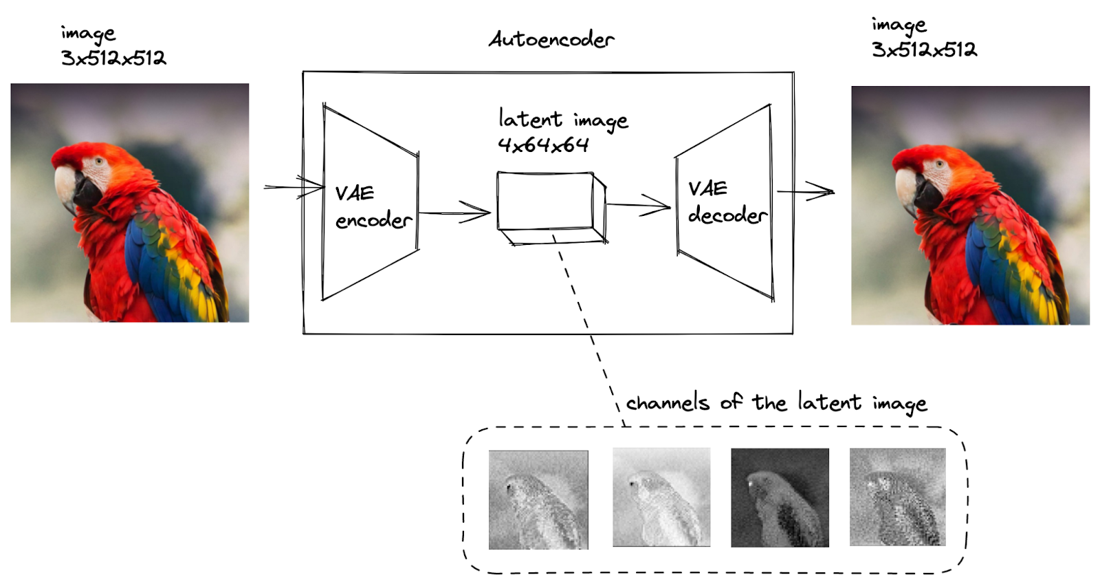
In the diagram, the model transforms the original image, represented as a tensor of 3x512x512 dimensions (3 channels for RGB colors and 512 pixels height and 512 pixels width), to a smaller tensor of 4x64x64 dimensions, called a latent image, and then back.
In order to predict noise in an image, we use the U-Net model extended with the attention mechanism, as shown in the diagram below.
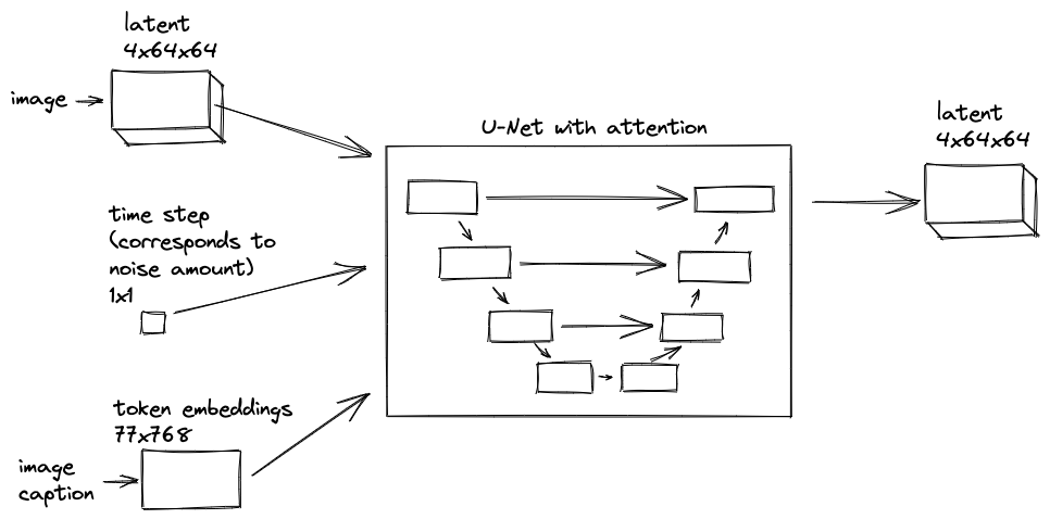
In the diagram, U-Net consumes:
- A latent image of 4x64x64 dimensions
- A time step scalar corresponding to noise amount as defined by the noise schedule
- An image caption represented as 768-dimensional token embeddings.
The non-image inputs are combined with the image in the model. The model produces a latent image of the noise at 4x64x64 dimensions.
We know what the U-Net model for noise prediction consumes and what it produces. Now the question is how such a model is trained.
Generating a training dataset for U-Net is shown in the diagram below.

In the diagram, we have a single image and a corresponding caption describing the image. From that, we generate many input-output training pairs for the model to train on.
To be more specific:
- We convert a single image in pixel space to a latent image and then create a couple of copies, each with a different amount of noise added to it (denoted as z+noise1, z+noise2, …). Apart from the latent image with noise, other elements that constitute training input are a time step scalar that corresponds to noise amount and a token embedding tensor (denoted as s). The embedding tensor is the same for each latent image with noise added.
- The training output (a.k.a. target) consists of a latent image of the noise (denoted as noise1, noise2, …).
Note that even though we consider one image-caption pair as input in the diagram, we use billions of such pairs in practice. Having such data, U-Net is trained to map the input to the output.
Inference, i.e. denoising
We know how the Stable Diffusion model is trained, i.e. how the weights of the underlying models are adjusted to map the input to output. How is such a model with fixed weights used to generate images corresponding to prompts?
We do denoising in the latent space. To be more precise, we start with a latent image consisting of pure noise and then remove the noise step by step by following the noise schedule. This is shown in the diagram below.

In the diagram, in the initial step, we generate a latent image consisting of pure noise generated from a normal distribution. The U-Net model consumes this latent image along with a prompt and time step scalar and produces the predicted latent noise. Next, the scheduler module produces a slightly less noisy version of the latent image given the current noisy latent image and predicted latent noise (different schedulers have different ideas on exactly how to do this; more on that in a moment). This gets repeated a number of times (e.g., 20 steps) until we get a latent image that doesn’t contain any noise. In the end, we transform the current latent image to an image in pixel space using the VAE model.
The scheduler consists of the following elements.
- The schedule maps the time step number to the noise level in the image.
- The sampler produces an image with a given noise level.
Side note 1. Let’s observe that the time step scalar ingested by U-Net is expressed as the training time step that U-Net was trained on. Typically we might have 1000 training time steps and only 20 denoising steps. Because of this, we need to map one to the other. In our example, denoising time step 10 would correspond to training time step 500.
Side note 2. Note that the whole process of denoising is deterministic, apart from 1) generating the initial latent image consisting of pure noise and possibly 2) calculating the latent image based on predicted latent noise. The latter might or might not be deterministic, depending on the scheduler used. To go a bit more into detail, let’s consider individual elements of the process:
- VAE – it uses randomness only when encoding, and encoding isn’t done during denoising
- U-Net – deterministic
- Scheduler – some schedulers are deterministic, and some are not. The default one used in diffusers, i.e., PNDM, is deterministic.
Denoising interpretation
Now let’s consider an interpretation of the denoising process, which will give us additional insight. Denoising can be interpreted as finding the closest point on the manifold of sensible, latent images. By “sensible,” we mean images similar to the ones seen during training. This is like an optimization task where the predicted noise corresponds to the gradient, a.k.a. the direction in which we need to go, and the scheduler uses this information to calculate the next latent point/image. The original idea comes from ordinary differential equation (ODE) solvers.
This is shown in the diagram below (a “Pikachu playing banjo” prompt is used).

In the diagram, at the top, we have a starting latent image consisting of noise only. In consecutive steps, a scheduler generates images that are closer and closer to the manifold of sensible images by subsequently removing noise from the image. We have two paths shown, each one corresponding to a different hypothetical scheduler. Each scheduler has a different idea of how to move the image closer to the manifold. As a result, scheduler 1 takes more steps and a less direct path, while scheduler 2 takes a smaller number of steps with a more direct path. Each scheduler produces a different final image since it lands in a different place on the manifold of “sensible” images.
Extensions and applications
We have shown how the core of the algorithm works; now, let’s take a look at some extensions and applications.
Visualizing denoising steps
During the denoising process, you might want to see what would happen if we jumped from the current noisy latent image straight into the whereabouts of the manifold of sensible images. This is how the denoising process is often visualized in showcases online.
You do it by performing the following calculation: latent_after_jump = noisy_latent – sigma * predicted_latent_noise, i.e., we take the current latent and remove predicted noise multiplied by the assumed current noise level as specified by the schedule.
As an example, see the table below. The table shows the current latent and the latent after the jump for a given denoising step (prompt: “Pikachu playing banjo”, 20 iterations).
| Step | current latent decoded with VAE | latent after jump decoded with VAE |
| 1 |  |  |
| 2 |  |  |
| 3 |  | 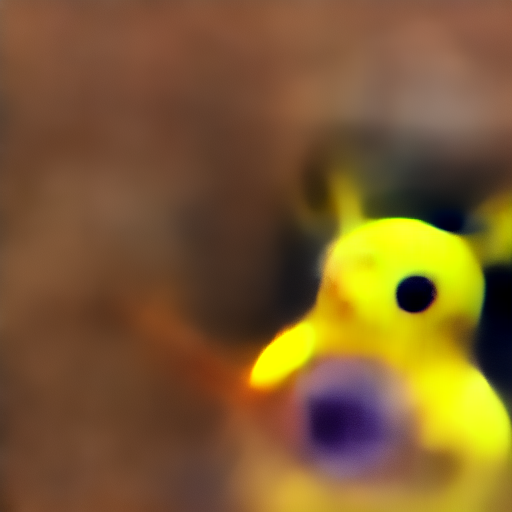 |
| 4 |  | 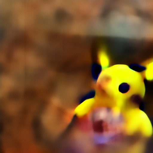 |
| 5 |  | 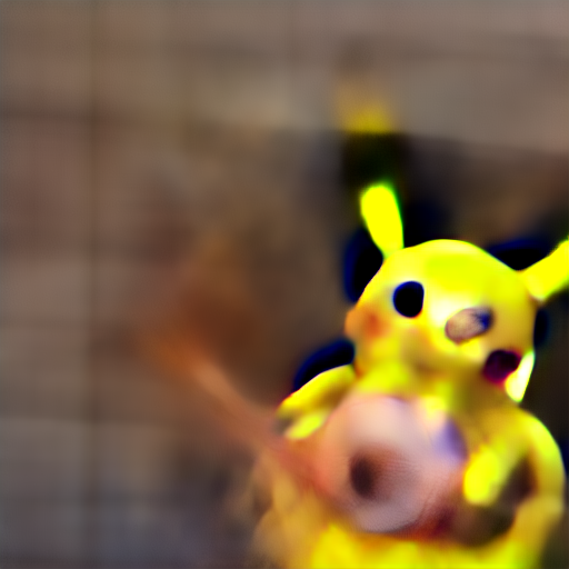 |
| 6 | 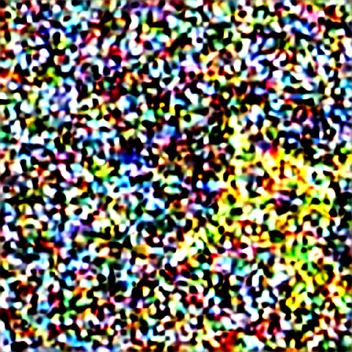 | 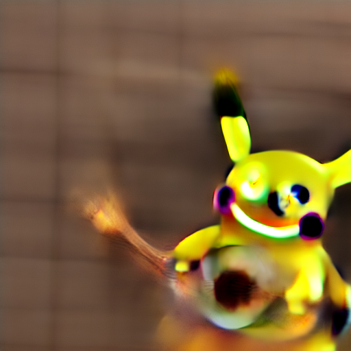 |
| 7 | 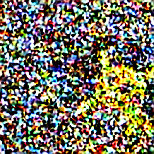 | 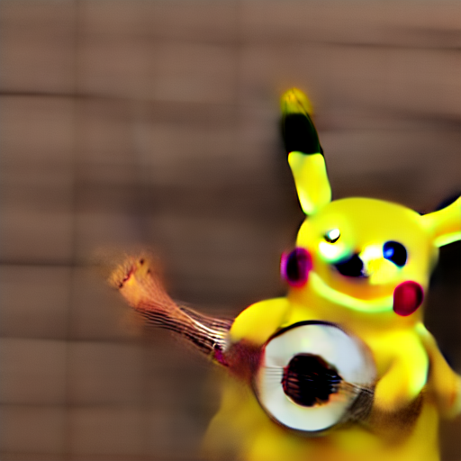 |
| 8 | 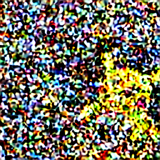 | 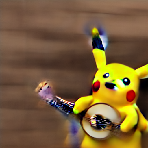 |
| 9 | 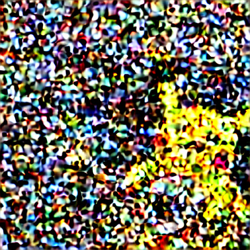 | 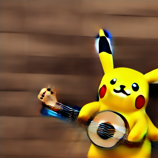 |
| 10 | 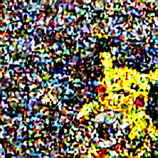 | 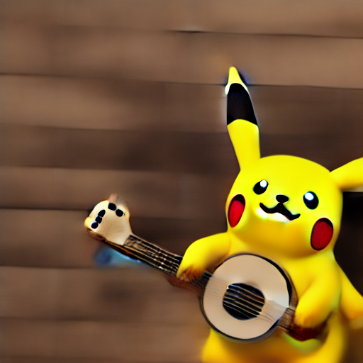 |
| 15 |  | 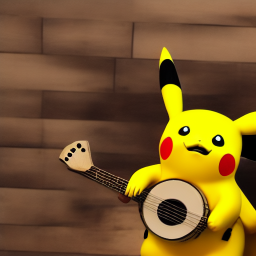 |
| 20 |  |  |
One can see that jumping at the beginning of the process, when you’re far away from the manifold of sensible images, produces images of low quality, while jumping at the end of the process produces images of high quality.
Guidance scale and negative prompt
Let’s inspect a standard extension of basic Stable Diffusion that allows for better control over the produced images. It uses two parameters: guidance scale and negative prompt. What are they?
- Guidance scale – the larger the value, the more closely the image follows the text prompt, usually at the expense of lower image quality (the default value in diffusers: 7.5)
- Negative prompt – text describing what we don’t want the picture to represent
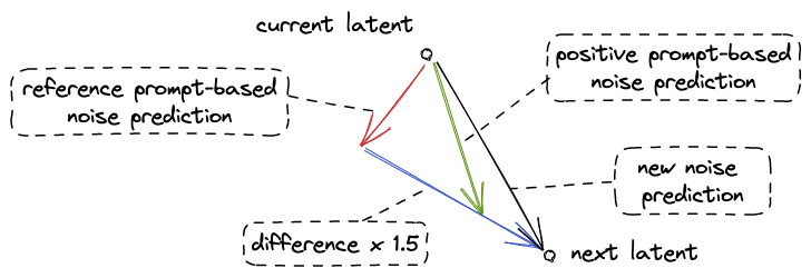
How do they affect the denoising process? In each denoising step, we do the following.
- Generate the noise predictions separately for the following two prompts.
- Positive prompt (called prompt and text in diffusers code) i.e. a description of what we want to see in the image.
- Reference prompt (called uncond in diffusers code) which is either a negative prompt describing what we don’t want to see in the image or an empty string if we don’t want to specify such information.
- Calculate the difference between these two predictions and move from the one based on the reference prompt in the direction of the one based on the positive prompt by guidance_scale amount, with guidance_scale=1.5, for example. This is the corresponding code from diffusers (with variable names changed):
- noise_prediction = reference_prediction + guidance_scale * (positive_prediction – reference_prediction)
The larger the guidance_scale, the more we move away from an image corresponding to the reference prompt.
This is shown in the diagram below (with guidance scale=1.5).
Tidbit: Negative prompt is an unofficial modification in Stable Diffusion 1.5. Apparently, it was first introduced in the popular Automatic1111 Stable Diffusion Web UI (see automatic1111 Web UI wiki and stable-diffusion-art.com website)
Side note: We use the negative prompt instead of simply using negative expressions in the normal prompt since the CLIP language model used in Stable Diffusion might not understand the negative expressions that are given in the positive prompt. For example, if we use the prompt “portrait photo of a man without a mustache,” the “without” word might be completely ignored. (see stable-diffusion-art.com website).
Image-to-Image
Let’s consider an interesting application of Stable Diffusion that allows for turning a drawing or a sketch into an oil painting/photo etc., called Image-to-Image.
An example with a sketch on the left and a photo-like quality image on the right is shown below (prompt: “cherries on a plate, high-quality artistic photo”).
 |  |
Steps of this method:
- encode the image into latent space
- add some amount of noise (to move it away from the manifold of sensible images)
- run the denoising process with some guidance text
As a result, you get an image with a composition similar to the original one.
Inpainting
Another area of application of Stable Diffusion is inpainting. In inpainting, we use a mask to mark a part of the image we wish to be replaced with something else.
An example is shown below (based on diffusers documentation).
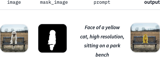
How does this method work? In general: extend the input latent image by adding additional channels with: 1) mask and 2) masked original latent image.
This extended latent image is shown in the diagram below (the images in the diagram come from diffusers documentation).
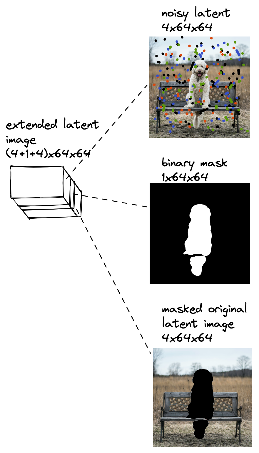
During inference, we run the denoising process as previously, but we use this extended input for U-Net instead of using only the noisy latent as input. The noisy latent initially consisting of noise only gets denoised in consecutive time steps, but the binary mask and masked original latent image stay the same.
Side note: If you want the inpainted area to resemble the corresponding area in the original image, you can apply the approach used in Image-to-Image as previously described.
Tidbit: Note that both the binary mask as well as the masked original latent image are images in latent space. They are transformed into latent space as follows in diffusers.
- The binary mask is simply a scaled-down version of the mask from pixel space.
- The masked original latent image is the masked original image converted into a latent space-based representation by VAE. This conversion involves randomness since VAE does sampling from a normal distribution when doing so. In the code it looks like this: self.vae.encode(masked_image).latent_dist.sample(generator=generator)
The training is done by fine-tuning of the standard Stable Diffusion model. For the fine-tuning stage, we produce a training dataset by masking random parts of original images and the model’s task is to reconstruct them.
Addendum
Here we present some additional details about the algorithm and its implementation.
U-Net architecture
U-Net architecture used in Stable Diffusion is shown in more detail in the diagram below.

Turning text into token embeddings
Transforming a caption into token embeddings tensor of 77×768 dimensions that is later ingested by U-Net (based on [2]) is shown below.
An example diagram:

Steps:
- Turn caption into token indexes, e.g. “pyramids in Egypt” -> “py”, “ramids”, ” in”, ” Egypt” -> 324, 134, 3422, 34
- Pad the text at the end with indexes corresponding to “empty” token to get 77 tokens, e.g. 324, 134, 3422, 34 -> 324, 134, 3422, 34, 0, 0, 0, …, 0
- Map token indexes into embeddings (vectors of size 768) using a fixed map coming from the language model.
- Each of the 77 tokens has a fixed position embedding (learned or not) coming from the language model. We add these embeddings to get a 77×768 token embedding tensor.
- This embedding tensor goes through a transformer model to generate a new 77×768 token embedding tensor. That is inputted directly into cross-attention modules in U-Net.
Side note: The division of the text into tokens and token indexes given above is made up. These would be different in a CLIP model used in a real algorithm.
Scheduler and schedule
The scheduler from the diffusers library, e.g. LMSDiscreteScheduler, is a sampler combined with a schedule.
It uses a set_timesteps() method which sets a new number of time steps to be used during inference/denoising. You can check how these new steps are mapped to the original training steps by accessing scheduler.timesteps and check the amount of noise at each of these steps by accessing scheduler.sigmas [2]. For example, if the training time steps number was 1000, we could have:
| > scheduler.set_timesteps(15) > print(scheduler.timesteps) [999.0000, 927.6429, 856.2857, 784.9286, 713.5714, 642.2143, 570.8571, 499.5000, 428.1429, 356.7857, 285.4286, 214.0714, 142.7143, 71.3571, 0.0000] > print(scheduler.sigmas) [14.6146, 9.6826, 6.6780, 4.7746, 3.5221, 2.6666, 2.0606, 1.6156, 1.2768, 1.0097, 0.7913, 0.6056, 0.4397, 0.2780, 0.0292, 0.0000] |
The schedule defines how sigma depends on the time step during denoising. An example denoising schedule with 20 denoising steps is shown in the diagram below.

Further reading
Main sources:
- [1] diffusers library v0.15.1 from Hugging Face – source code
- [2] Jonathan Whitaker: fast.ai’s “Practical Deep Learning for Coders” 2022 course, lesson 9A 2022 – Stable Diffusion deep dive
- [3] Jay Alammar’s blog post: “The Illustrated Stable Diffusion”, 2022-11
- [4] Ho et al.: “Denoising Diffusion Probabilistic Models”, 2020 – the bedrock for all diffusion models that everyone refers to, a.k.a. the “DDPM paper”
- [5] Rombach et al. “High-Resolution Image Synthesis with Latent Diffusion Models”, 2022 – the “Stable Diffusion paper”
Additional sources:
- [6] Jeremy Howard: fast.ai’s “Practical Deep Learning for Coders” 2022 course, lesson 9: Deep Learning Foundations to Stable Diffusion
- [7] Hugging Face blog post: “The annotated diffusion model” – they show how to implement DDPM paper step by step
- [8] Hugging Face notebook: “Getting started with diffusers” – description of how the basic diffusion process works (without conversion to latent space nor text guidance)
- [9] Hugging Face’s blog post: “Stable Diffusion with Diffusers”
